


Georeferencing is a mapping technique where an image is overlayed on a map using ground control points (GCPs). These points link together the image and the map and provide a clean alignment. For this tutorial, I am using a map of North America.
Georeferencing involves transformations that yield different results on the map and the X, Y residuals. Before you begin, be sure to have your GCP’s. Simply overlaying the map on the basemap and connecting the points will cause major distortions with the map title and legend. When I first made this mistake, I used third-order polynomial transformation; while everything seemed correct at first, unmanageable technical issues popped up.
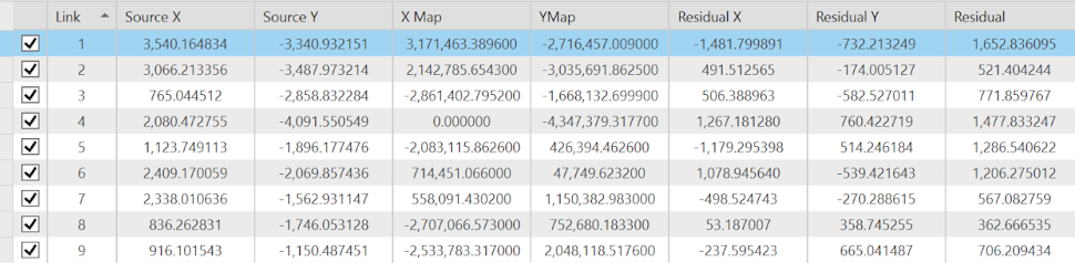
Here, I use the Similarity transformation. The 1st-Order Polynomial transformation requires three control points. When I have only three links selected using the 1st-Order Polynomial transformation, the Residual X and Y become 0. When I select a fourth link, the residuals change. With a fourth link selected, the Residual X increases while the Residual Y decreases compared to a full checked table.
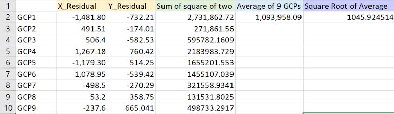
It is important to calculate the RMSE of the GCPs. I can do this by copying the X and Y residuals into an Excel spreadsheet; the number comes to 1045.92. I use the column to their right to perform a calculation called “sum of squares”, or in Excel, “sumsq”. Let’s say I want to calculate the sum of squares for GCP1: I would type =SUMSQ(B2,C2) into D2. After repeating this function for all nine rows, I find the average by using =AVERAGE(D2:D10). Afterwards, I calculate the square root of the average by using the expression =SQRT(E2).
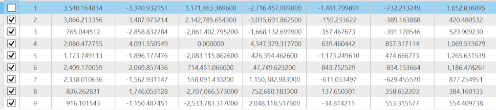
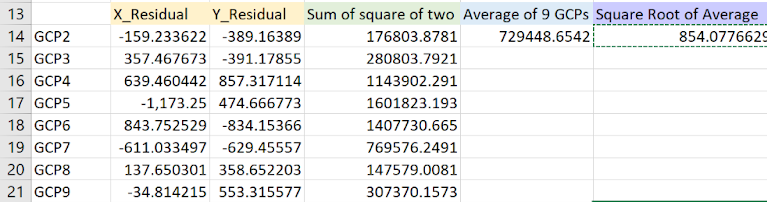
It is ideal to have low residuals to maintain an accurately georeferenced map. A high RMSE indicates potential issues with the precision and accuracy of the map and satellite imagery. If I were to remove a single GCP from the sheet, it would be GCP1, since it has the highest residual. After recalculating the RMSE with GCP1 removed, I find it drops from 1045.92 to 854.077. First, I uncheck GCP1 from the control point table in ArcGIS Pro; this should noticeably shake up the numbers. I copy GCP2 to GCP9 into Excel and perform the same functions (as detailed in the previous paragraph), except with different lettering and numbers associated with the fields. While removing a high residual GCP will lower the RMSE, it is sometimes better to accept it; the inaccuracy may lie in the map.
You may notice the lines of longitude and latitude splayed across the map; while they may seem distracting, they help with GCP creation. Nevertheless, georeferencing without lat/long lines requires an alternative method. Let's say I have a large-scale map of Los Angeles. One way to go about this is by overlaying the image onto a basemap. I can georeference by changing the image's scale and rotation, and if necessary, moving it around. From there, I can connect the image and the source by ensuring the two points maintain precisely the same location in relation to one another. Be sure to check whether the projections match before using this method.
I can record the coordinates of the GCPs with a GPS. Since they are initially recorded in degrees, minutes, and seconds, they require conversion to decimal degrees. This will yield latitude and longitude data. After performing this conversion (using an online tool), I can tidy up the data with a spreadsheet. After a quick import into ArcGIS Pro, I can display X and Y data.
If I repeat my georeferencing process with my GCS_WGS_84 GCPs, I get similar results towards the end of the georeferencing process. If the points do not have a suitable coordinate system, they will result in inaccuracies and possible distortions. Near the beginning, the image may not be adequately aligned (especially with the first several points). However, as it becomes more aligned due to the georeferencing, the distance between the GCPs and the selected locations on the lines of latitudes and longitude will become closer.